Deep learning plays a key role in modern AI (Artificial Intelligence) and machine learning. It uses a series of ‘neurons’ structured in layers to break down the data and extract the outputs we need.

These neuron-layer complexes that we’ve described are called neural networks, or ANNs (artificial neural networks).

As you may have guessed, this structure of neurons is something like how the neurons in our brains help us learn as humans. The analogy isn’t perfect but some of the ideas of deep learning are in fact borrowed from the way human brains function.

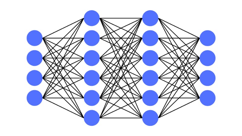
The above image is a visualization of a neural network. The blue circles in the picture each represent a neuron. The neurons lined up vertically are the layers. The lines that join the neurons are connections that play a big role in processing the data.

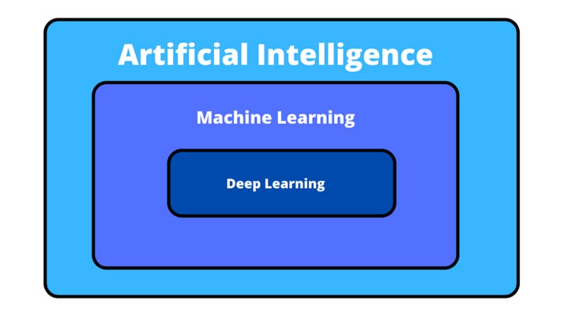
It’s common to develop misconceptions regarding the difference between deep learning, machine learning, and AI. Although sometimes these terms are used interchangeably, deep learning actually describes a particular way of training machine learning models making it a part of a bigger world of machine learning. Machine learning (a way of allowing algorithms to figure out how to predict outputs) is itself a subset of AI. Anything that provides un-human things with a way to do human stuff, in general, comes under AI.

We will be breaking down the approach that deep learning takes to allow machines to gather insights from data. This post will address neural networks in such a way that the essence of this machine learning methodology is covered. Some of the math will be brought up, yet it will be explained and its place in deep learning will be justified.

Overview of Neural Networks

As we’ve discussed, deep learning is a way of training computers to predict outputs based on certain specified inputs. This is done by passing input data through layers of ‘neurons’ which each manipulate the data and pass it on.

Neurons (in a deep learning sense) are entities that hold numerical values which influence how the data is passed on and outputted. Sometimes these neurons are also called nodes.

Each neuron, and in effect, each layer does its own thing to the input as the data moves forward through the network.

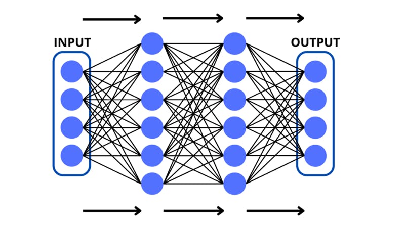
The network begins at the input layer which stores an input that the network needs to make a prediction for. The input is read by the layers in the neural network as a list of numerical values, called a vector or a tensor. The only difference is that vectors are one-dimensional lists (single lists of quantities) however, tensors can also be multi-dimensional and arranged as grids.

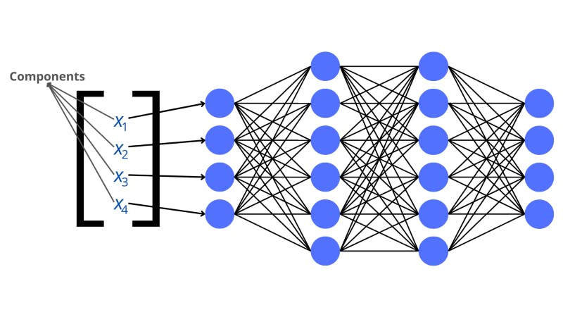
Each value in the input vector corresponds to a neuron in the input layer. These values in the vector are called components.

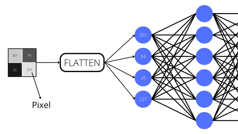
For instance, if the neural network were tasked with computer vision (analyzing visuals to make predictions) for grayscale images, then an input image would be flattened into a vector. Each neuron in the layer would represent a pixel with a value between 0 and 255 (this is how greyscale images are generally stored).

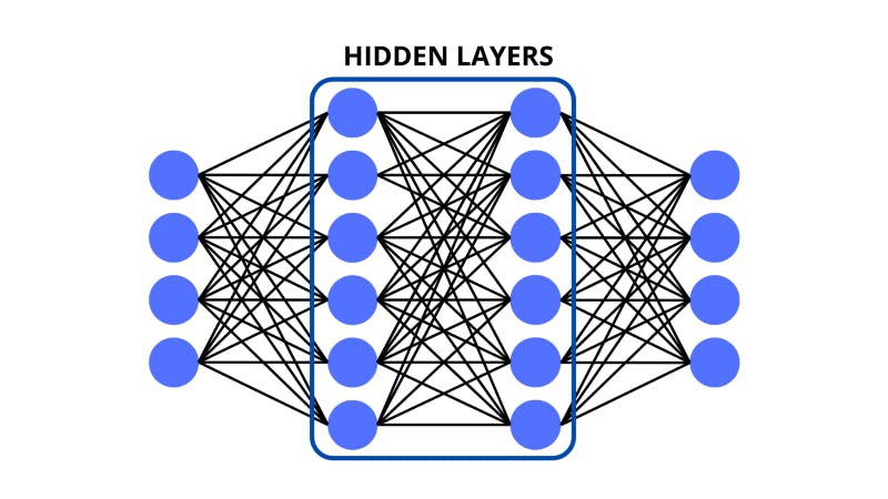
Following the input layer, the data is crunched-up by the neurons in the middle layers. These layers between the input and output are also commonly called the ‘hidden layers’. They do some math on the data and pass the processed inputs on. We will go into the details of these operations later on.

For now, it’s important to understand that the bulk of the processing of neural networks is done in the hidden layers. There can also be as many hidden layers with as many neurons.

The hidden layers feed the crunched-up data into the output layer (the last one) which can represent different things depending on the type of model that is being made. There could be a single neuron that predicts a certain numerical value, this would be called a ‘regression’ model. Or there could be multiple neurons in the output each standing for a probability of the input belonging to a certain class — this would be a typical ‘classification’ model.

But how does a neural network reach the state of being able to make such complex predictions? How does it know what math to do to the vector input so it is progressively morphed into the output we wanted?

This is another place that neural networks take a cue from us humans: the neural networks learn with thousands of examples from data. The input values, commonly called the ‘features’, are fed into a randomized network. The network’s internal knobs and dials are arbitrary at the beginning so the deep learning model doesn’t perform very well. We tell the neural network the correct answers and it discerns how close it was. Depending on this, it tweaks itself to perform better. We call this process ‘training’ and as we repeat it, the neural network becomes a trained machine learning model.

The Inner Workings: Weights, Biases, Activation Functions

The numerical value of a neuron that’s used by the network is called its activation. The neuron activations in the network depend on various factors. These include the activation of the previous neurons it’s connected to, the weights between the linked neurons, a bias, and the activation function.

Let’s break these down.

So, what really ties the neuron that we’ve selected to the other neurons in the input? We visualize it with lines, but what do the lines mean?

For a neuron to be linked with another, the activation of the first neuron should influence the activation of the next. There also needs to be a unique weight associated with the connection between the two neurons that impacts the activation.

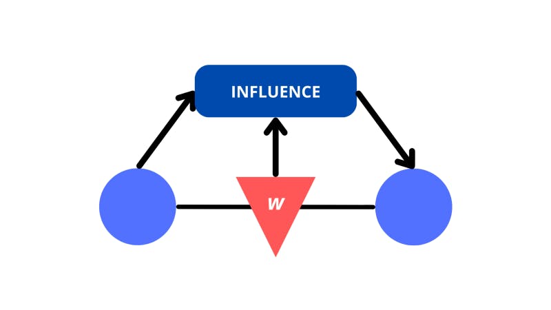
A high-level view of what connections between neurons mean

Now, take the following neuron in the following neural network:

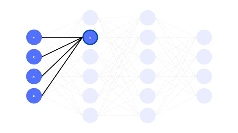
The x1, x2, x3… xn are activations of neurons in the input layer. They also represent the different components (items of a vector) in the input vector. Each activation in a layer is thus a component of the vector representing the layer.

In the next layer, the neuron with activation a is connected to all the neurons in the previous layer. This configuration is known as a dense layer (where the neurons from one layer are all attached to the neurons in the previous layer). The dense layer is one of the main types of layers used in neural networks.

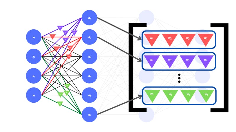
As we mentioned before, there need to be weights corresponding to each connection between the neurons.

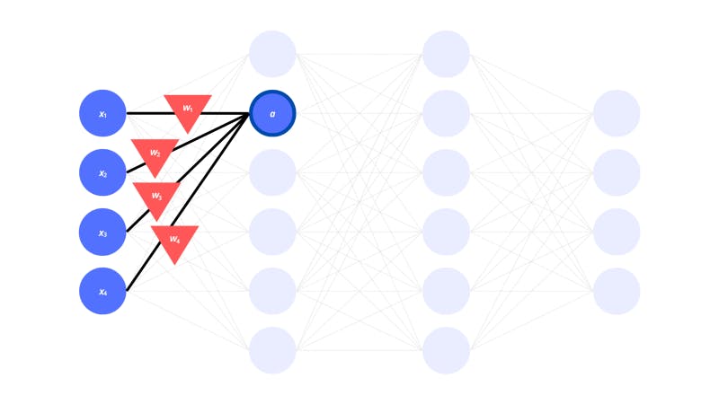
The triangles in the image above represent the weights. But how do the activations of the previous neurons and the weights for the connections actually influence the next neurons?

The weights are multiplied by the input activations of the corresponding neurons in the previous layer. All these products are added up to get the activation of a single neuron in the next layer. There is also a bias value to be added on top of all this.

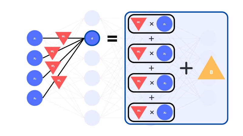
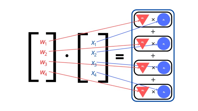
In a linear algebra sense, the computation of these individual neurons is a dot product between the input vector and the vector of weights. Except there’s also an extra bias we add on top.

A dot product is seen as the multiplication of two vectors outputting a single number. When taking a dot product, you multiply all the components of one vector with the matching components in the other vector. By adding all the results up, the output is a single number.

We repeat this process of finding the dot product and adding a bias to get the value of the neurons in the second layer. Now, if we arrange the results in a vector that represents the layer that we’re working out, we’ve effectively performed a linear transformation on the input vector. This is another term taken from linear algebra. A linear transformation is where we map (or transform) a vector into another vector.

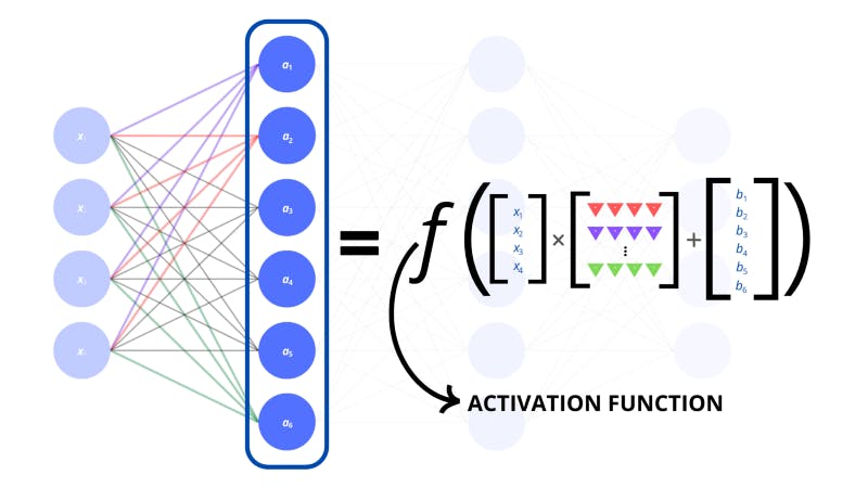
The way we transformed our input vector was by multiplying it with a matrix of weights. Woah, matrix? Remember we discussed tensors? Well, matrices are two-dimensional tensors (called tensors of the second rank). They are arranged as grids (or a list of lists). The weights for the entire input layer to individual neurons in the hidden layer can be represented by vectors. There are multiple vectors of weights for each neuron in the hidden layer which we can stack to form a single matrix.

A matrix can be thought of as a set of instructions to transform a vector. A unique matrix will transform a vector in its own special way. Visualized in a vector space (a plane) a matrix will manipulate (or transform) a vector in the same manner. For example, a particular matrix will always rotate a vector by some angle, no matter the position on the vector space.

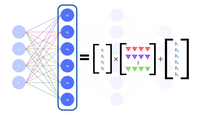
The linear transformation of the input layer gives us the vector for the next layer

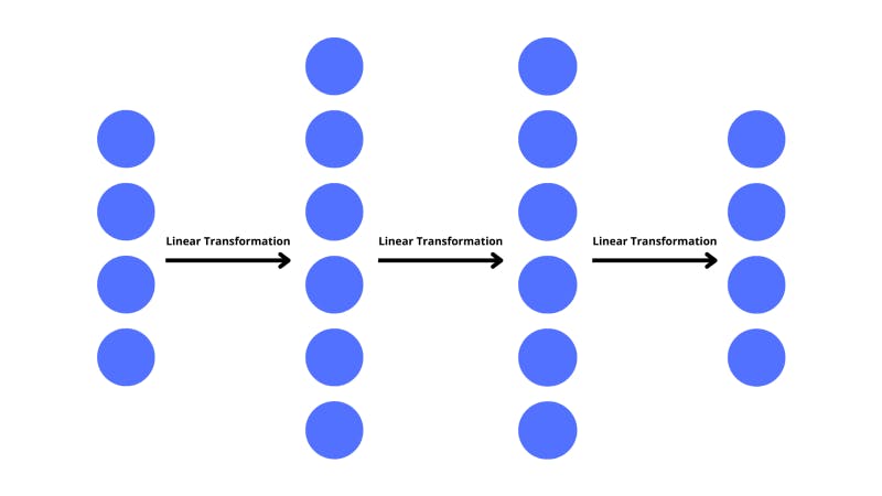
The only two operations that we performed were multiplication and addition which are linear. If the math we did were to be graphed, we would see straight lines. There were no complex operations that would’ve added any curvature to the visualization of the operations. This is why we call the transformation linear.

Thus, we have a transformation of a vector that is linear in a vector space — a linear transformation. When going from one layer to the next, the data (as a vector) is just transformed by a unique matrix of weights.

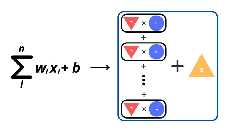
In reality, the process for computing the activation of a neuron (taking the dot product of the input vector and a vector of the weights) may be represented with some pretty scary symbols and math.

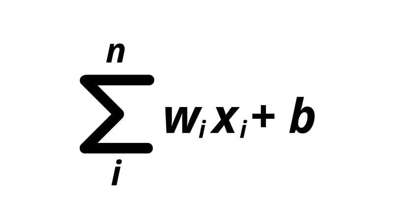
The ‘sigma’ symbol is used for summation operations. These types of operations enable us to denote the adding up of expressions in a sequence. The i beneath the sigma tells us the index variable which is what increases every time we add another expression to the sum. The n on top is the maximum value for i after which we need to stop increasing. For my friends from the programming world, just imagine the summation as a “for loop”.

In the expression, the w means the weight for the specific neuron connection, and the x is a value from the input vector.

The formula on the right of the sigma is the expression that we need to add up based on our index variable. In this case, for every ith x in the n neurons, we multiply it by the ith w. We sum up all these weight-input products. In the end, a bias (B) is added.

Thus, this summation formula is just a condensed version of the extended expression that we went through before where we add up each neuron multiplied by a corresponding weight and add a bias at the end.

But the question may arise that if every single layer just represents a linear transformation, then there’s no need for multiple layers. The multiple linear transformations could easily be adjusted into a single transformation between two neurons.

This is where activation functions come in. These are there to mix things up, specifically, they add non-linearity to the model which helps us compute more complex data. There are several activation functions that are all helpful for different kinds of operations.

The computation of the activation which we just went through now also goes through an activation function.

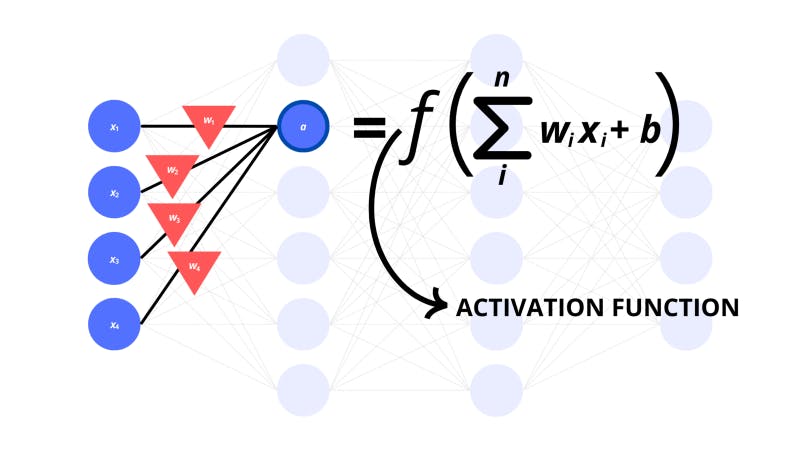
To express this for the whole layer, we can put an activation function around the linear transformation. This way, we know to apply the activation function to every single component of the resultant vector.

Developers specify the activation function for different layers that they think would be helpful.

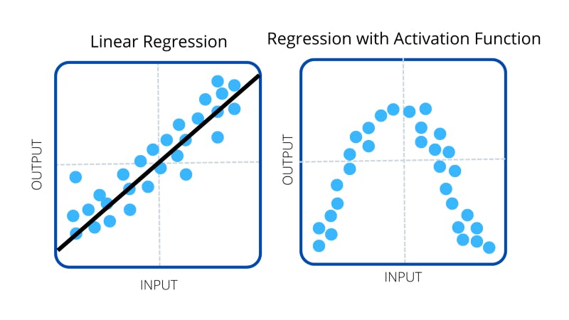
Sometimes we want to create models that predict in a linear fashion by trying to estimate numerical data with a linear transformation. These are called linear regression models and when geometrically interpreted, they use straight lines to model the data. We know to use this type of model when there’s a clear relationship between the input and output (like the output increases at a constant rate when the input increases). In these cases, we don’t add an activation function to the layers. However, if the numerical data is non-linear and its graphs involve some curves (non-linear aspects), then we do use these activation functions. If the data is not numerical at all and we’re dealing with classification models, then we also don’t use activation functions.

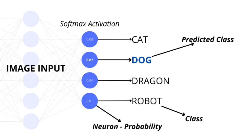
One of the activation functions which is used for classification models is called softmax. This adjusts the final layer to represent the probabilities of the input belonging to a certain class where each neuron represents the classes. Developers generally set this activation for the final layer of a neural network to classify the input.

Another popular activation function called sigmoid squeezes the activation of a neuron into a number between 0 and 1.

We are not going to go into the details in this post. These functions can be quite complex but you don’t need to understand these completely to build your own deep learning models. To be clear, activation functions are used to capture data that doesn’t follow a linear, obvious pattern.

It’s important to understand that a single connection between two neurons, is insignificant, but how the connections eventually form a bigger picture is paramount.

Training: Evaluation, Tweaking, Trying Again

So far, we’ve talked about how a neural network works — but how it’s trained is also really important.

Initially, the network is completely random. So the first time it tries predicting an output for an input in a dataset, there’s no hope.

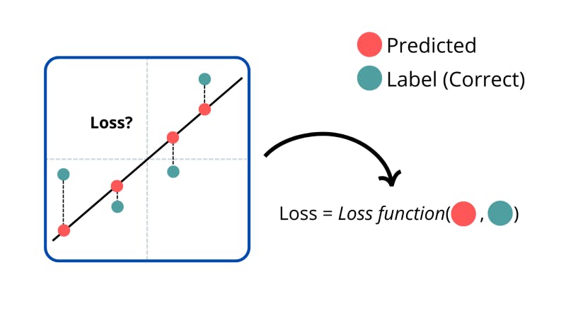
Then, the network does something amazing; it measures how bad it sucked. This is known as calculating the ‘loss’, or sometimes also called the ‘cost’. This is calculated with mathematical functions which measure how close its outputs (the predictions) were to the labels (the correct outputs).

If we were building a linear regression model (where we predict the output for some inputs with a linear graph) then we would see how far the correct outputs were from our model.

The untrained model then does something that’s arguably even cooler; it improves. The weights and biases in the network are adjusted. The network computes what’s called the ‘gradient’ of the loss function with respect to all the weights. The gradient is the change in a function’s value with a tiny change in the input. If this change is negative in the loss function that means that the loss is going down and we’re going in the right direction. Eventually, by changing the weights and looking at the impact on the function, we can reach the lowest value of the loss function and the highest accuracy.

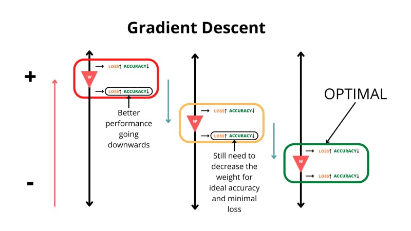
The neural network looks at what happens when it increases and decreases the value for a certain weight.

The algorithm in charge of finding the lowest point in the loss function is known as gradient descent. But how are we supposed to find the gradient of the loss function with respect to all the weights in the network? This is done with a process called backpropagation which goes back through the network to find which weights and biases need to be changed for a decrease in the loss.

Backpropagation and gradient descent are amazing algorithms in charge of the learning process for neural networks. However, the math behind them gets pretty complicated. The explanation would make for a post of its own. Again, to just develop neural networks this information isn’t necessary, you really just need to grasp the purpose of backpropagation and gradient descent.

Essentially, when backpropagating the network has a look at what impact certain weights are having on the neural network’s performance. It computes the gradient of the loss with respect to the weights. Gradient descent navigates a way to reach the bottom of the loss function using the gradients from backpropagating.

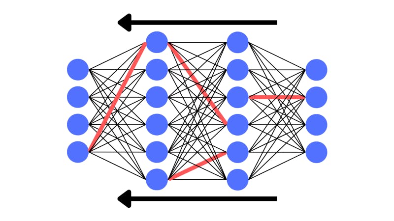
The network has picked certain weights to alter once it has backpropagated

Gradient descent on its own describes a way of finding a minimum value of a function. But there are special gradient descent algorithms that locate the minimum value. These are called optimizer functions. They need to adjust a hyperparameter called the ‘learning rate’.

Hyperparameters are values that are parameters in charge of the training process of a network. The learning rate describes how the neural network goes about changing the weights and biases to minimize the loss. If it takes big chunky steps with big changes then there is a high learning rate. On the other hand, if there are tiny, gradual steps the learning rate is lower. The optimizer function adapts the learning rate to ensure we don’t get stuck making too small, or too big changes in the network.

After this, the neural network tries predicting the output for another input by propagating the data.

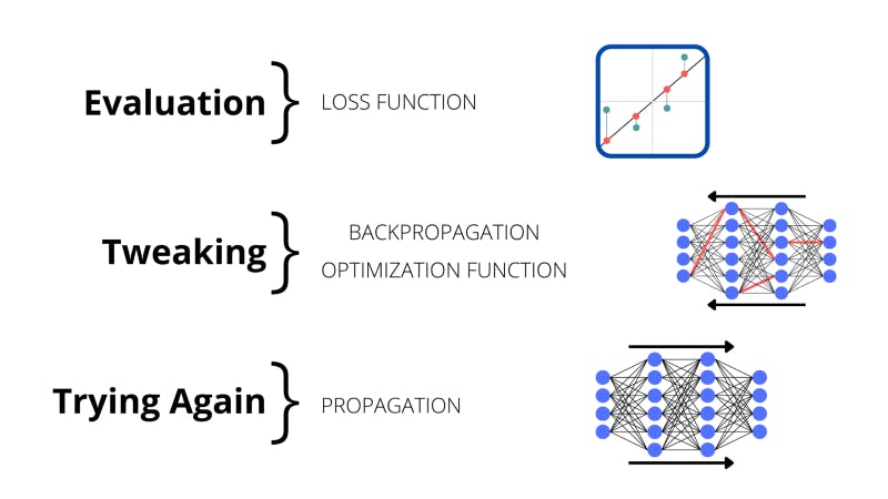
This method of the model evaluating, then fixing itself, and finally trying again is how the neural networks improve; this is essentially the process that trains computers to drive cars.

Once these processes of calculating loss, backpropagating, and propagating are repeated enough times, we are led to an accurate deep learning model.

Summary

In this explainer, we’ve seen that deep learning models make predictions about inputs with neural networks. The networks are made up of neurons arranged in layers. Starting from the input, each layer transforms the data. Eventually, this processed data is handed over to the output layer which represents the answers we needed.

Through a process of training, the neural network adjusts its internal variables in charge of the operations crunching up and transforming the data. Its accuracy improves as it keeps making predictions and trying gain.

Hopefully, this post was beneficial to your understanding of deep learning and neural networks. Deep learning is something that many of the AI technologies of this day are based on. Once you begin to grasp the fundamental ideas behind the neural networks of deep learning, you can even start constructing your own models that solve real-world problems.